
Collective phenomena far from equilibrium

General aspects
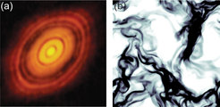
Symmetry breaking and pattern formation are striking collective phenomena which can be observed in many systems far from thermal equilibrium. Well-known examples are the swarming of starlings [1,2], patterns in bacterial colonies [3], laning in colloidal suspensions [4], thermal convection [5,6], or the stop-and-go waves in a traffic jam [7]. A primordial example is the clustering of the granular dust in the accretion discs surrounding young stars (cf. Fig. 1), which eventually leads to the formation of planets, such as Earth. Common to all these systems is that
- they are dwelling far away from thermal equilibrium
- they consist of a very large number of similar sub-systems
- these sub-systems are not in thermal equilibrium themselves.
The nature and complexity of the sub-systems varies considerably. In the accretion disc, these are the dust particles whose mutual collisions are dissipative because some of the impact energy is lost into their internal atomic degrees of freedom. On the other hand, there is almost no limit to complexity, as seen from the 'participants' in microbial turbulence [8,9], swarming of mammals, or traffic jams. Similarly, the character of the mutual interactions varies dramatically. Nevertheless, striking similarities in the collective behavior of widely different types of constituents have been observed. This naturally prompts the question why at all structure emerges from previously homogeneous systems, and whether there are general principles governing their evolution. Resorting to the example of planet formation, it becomes clear that these questions touch on the very basis of our existence.
 A planetary accretion disc around the star HL Tau (image taken by Atacama Large Millimeter/submillimeter Array (ALMA)). The dark rings are depletion zones indicating orbiting young planets which collect the granular dust in these regions. (b) Clustering in a granular gas, investigated by direct numerical simulation of a dissipative Navier-Stokes equation.")
In search for a conceptually general treatment of such systems, which eventually may reveal overarching principles governing their behaviour, it suggests itself to start from their textbook counterparts. Collective phenomena in condensed matter consisting of simple sub-systems, such as atoms, molecules, or colloidal particles, can be considered well understood, at least sufficiently close to equilibrium. The validity of microscopic equilibrium (Kolmogorov criterion [10,11]) enables the application of classical statistical physics, through which a suitable free energy density can be written down. In general, the steady state corresponds to the minimum of the free energy of the system.
The quest for analogous minimization principles governing non-equilibrium steady states (NESS) has a long history [12]. While for systems with microscopic equilibrium it is established that the NESS corresponds to a minimum of entropy production [12-14], the question to which extent this holds also away from microscopic equilibrium is still not settled. Claims that extremal entropy production serves as a general principle for systems far from thermal equilibrium [15,16] have soon been challenged [17], later proven wrong [18,19]. More precisely, it was shown that if there is a functional which generally has an extremum in the NESS of the system, it cannot be expressed in terms of entropy production. This does, however, not preclude the existence of more general functionals, which are based on other quantities characterizing the NESS.
 The dynamics of any system can be represented by transitions between its possible states, which together form its state space. The arrows indicate these transition currents, which are determined from the transition rates and the occupation probabilities of the individual states by means of the master equation. (b) The Poincaré section describes the trajectory of a system in continuous state space by means of the sequence of its points of intersection with a suitably chosen plane. The cyclic character of the trajectory, or at least most of it, is thereby lost.")
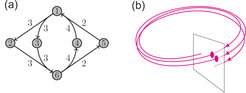
In order to introduce a powerful paradigm of looking at NESS, we consider first a discrete version of the system under study, which is represented in the space of all of its possible states (cf. Fig. 2a). In this picture, the dynamics of the system is governed by a master equation, which contains all transition rates between adjacent states. If there are no net currents in the NESS, the system is said to obey detailed balance. In that case, it is straightforward to construct a potential from the transition rates which is minimized by the most probably visited state.
In systems far from equilibrium, however, detailed balance is not fulfilled, such that this construction fails. It is interesting to note, however, that if we represent the system dynamics not by the states it visits, but by the closed cycles in the space of states which it can be conceived to dwell on, we find that the transformed master equation (describing transitions between cycles in state space) always fulfills detailed balance [20,21]. In a continuous picture this can be readily illustrated, as sketched in Fig. 2b. The well-known Poincaré section yields a transition from describing a system by its positions in state space to a description in the space of cycles in that space. Obviously, the currents connected to the cyclic trajectories are projected out, and the motion on the Poincaré plane has lost (at least almost) all cyclic character. It is rather reminiscent of a diffusive process, which fulfills detailed balance.
This suggests that in the space of cycles there should exist a potential which governs the dynamics of the system, in the sense of a 'free energy' which is minimized by the NESS. Unfortunately it turns out that the transition rates between cycles can be calculated only if the density in state space, i.e., the solution of the master equation in state space, is already known. This renders the transform to cycle space not useful for the master equation approach.
At first glance, one would think that a continuum description of the system, in terms of a Fokker-Planck equation instead of a master equation, makes things worse, because it just adds the complexity of having to deal with infinitely many states. However, it turns out that the Fokker-Planck picture offers a very promising line of attack. If we consider the drift field of the Fokker-Planck equation, we can say that the NESS will be strongly governed by the invariant manifolds of that field, if interpreted as a dynamical system. Hence the invariant manifolds (fixed points, limit cycles, limit tori etc.) are the important entities whose occupation probability yields all relevant information on the NESS. Interestingly, it turns out that we can compute the transition rates between adjacent cycles, at least in two-dimensional Fokker-Planck equations, by straightforward line integrals using only 'microscopic' information, i.e., the diffusivity field and the drift field. No a priori information on the solution of the equation (i.e., the density distribution in state space) is required. The central challenge is now to derive a general scheme which applies to arbitrary dimensions, including infinite dimensions. This would eventually provide a solution to the puzzle of constructing a general potential which governs processes like pattern formation and spatio-temporal chaos.
Some examples of collective behavior studied in our department
Aside from granular gases as a particularly simple type of systems far from equilibrium [22], we study agent-based systems of active matter. Our focus is on collective phenomena which are not easily predicted on the basis of the properties of individual agents and their mutual interactions. Simple examples are actively swimming microbes, such as the plankton in the oceans. Their collective behavior leads to clustering phenomena which are particularly complex due to the coupling to the flow of the seawater, both passively and by buoyancy coupling.
The substantial effect this coupling may have on collective phenomena can be well studied with active emulsions as a model system. Fig. 3 shows the swarming behavior of oil droplets of about 50 µm diameter which self-propel at typical velocities of a few µm/sec in an aqueous suspension of a suitable surfactant. Gradual solubilization of the oil in the surfactant solution provides the fuel for the self-propulsion. The diameter of the container is about 5 mm. One observes the emergence of a Cahn-Hilliard-type pattern leading to the formation of swarms with a characteristic dominant distance, λ. As the density difference between the liquids is varied by addition of D2O to the aqueous phase, we find that the swarming ceases as this difference becomes too small. In fact, the pattern is due to the formation of convection rolls with size λ, driven by the propulsion forces.
![Fig. 3 Formation of swarms in an aqueous suspension of actively propelling oil droplets [26]. The density of the aqueous phase, and thereby the density difference Δρ between the aqueous phase and the oil, was varied by addition of D2O. Clearly, the swarm formation goes away when the density difference is too small (i.e., of order one percent or less) demonstrating the crucial role of buoyancy coupling for these patterns to form. The length scale of the swarm pattern indeed turns out to correspond to the size of convection rolls in the aqueous fluid, driven by the self-propulsion forces of the droplets.](/3209005/original-1518437713.webp?t=eyJ3aWR0aCI6MTY5NiwiZmlsZV9leHRlbnNpb24iOiJ3ZWJwIiwib2JqX2lkIjozMjA5MDA1fQ%3D%3D--3b54fd75c3d653f22bd2406a58a450c8b2a0179b "Fig. 3 Formation of swarms in an aqueous suspension of actively propelling oil droplets [26]. The density of the aqueous phase, and thereby the density difference Δρ between the aqueous phase and the oil, was varied by addition of D2O. Clearly, the swarm formation goes away when the density difference is too small (i.e., of order one percent or less) demonstrating the crucial role of buoyancy coupling for these patterns to form. The length scale of the swarm pattern indeed turns out to correspond to the size of convection rolls in the aqueous fluid, driven by the self-propulsion forces of the droplets.")
![Fig. 3 Formation of swarms in an aqueous suspension of actively propelling oil droplets [26]. The density of the aqueous phase, and thereby the density difference Δρ between the aqueous phase and the oil, was varied by addition of D2O. Clearly, the swarm formation goes away when the density difference is too small (i.e., of order one percent or less) demonstrating the crucial role of buoyancy coupling for these patterns to form. The length scale of the swarm pattern indeed turns out to correspond to the size of convection rolls in the aqueous fluid, driven by the self-propulsion forces of the droplets.](/3209005/original-1518437713.jpg?t=eyJ3aWR0aCI6MjQ2LCJvYmpfaWQiOjMyMDkwMDV9--31012f45d389df5f9a3587c93ebb07d7539905b7)
 Formation of filament bundles in a Petri dish. b) optical micrograph of algal filaments moving in 2D, between an agar plate and a glass slide. Filaments move almost only along the path defined by their contour, with velocities of a few microns per second (the image is about 1 mm across). Their collective motion appears like traffic on a multi-line freeway. The topological defects in the pattern (circular and triangular voids) are stable over days.")
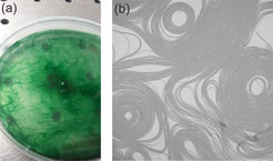
Microbes have of course more internal degrees of freedom than droplets, and therefore the emerging structures may be much more complex than what we see in Fig. 3. A fascinating example are filamentous green algae (cf. Fig. 4a) consisting of single cells which stack to create filaments many thousands times their diameter in length. By virtue of a so far unknown mechanism, these filaments move with respect to a substrate they are placed upon with a typical velocity of a few µm per second along the path defined by their contour. If these are constrained to two dimensions, their collective behavior shows up clearly. This is demonstrated in Fig. 4b, which shows an optical micrograph of filamentous algae squeezed between an agar plate and a glass slide. When observed in time lapse, these structures appear like car traffic on gigantic multi-lane freeways. The topological defects in the structure are very stable and last for days.
Collective behavior in socio-economic settings
The arguably most important question of our time is how Homo sapiens can organize a sustainable management of its ecological niche on planet Earth. Answering this question involves a tremendous amount of interdisciplinary research on all relevant aspects of socio-economic systems. Almost all of these classify as collective behavior far from equilibrium. Based on our studies of the above mentioned model systems, it is hence of central interest to investigate how game theoretical and other mechanisms characterizing the interaction of living agents modify collective behavior.
A simple way to define a formal measure of intelligence can be gained from observing chess players. Strategies can be generally cast into saying that a player always tries to maximize the number of options for future moves. In an arrangement of many identical agents, one may analogously define that each agent tries to move such as to maximize the number of random walks of a predefined length it can perform without running into another agent. This is just a single number characterizing the 'comfort' with respect to the freedom to move around, at a current position within the other agents. The logarithm of this number has been termed the 'causal entropy' [27], and the derivative of this entropy with respect to the agent’s position is equivalent to a force acting upon the agent. The predefined length of the random walk can be regarded as the size of the 'cognitive map' the agent uses to probe its surroundings, and hence defines a measure of 'intelligence' (similar to the number of moves a chess player can think ahead).
 of these hypothetic random walks, i.e., by the size of their cognitive map. The so-defined intelligence is small in the left picture and increases from left to right.")
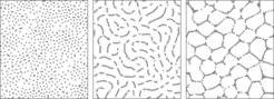
If we simulate a large number of such agents and vary their intelligence as defined above, we indeed obtain strongly variable collective patterns (cf. Fig. 5). While for no or only small intelligence we find random arrangements (left), increased intelligence results in the formation of long filaments (center) or even honeycomb-like patterns (right). Obviously, the impact of the intelligence of the actors on their collective behavior is substantial.
Finally, we treat demand-driven ride sharing systems with techniques of statistical physics. These are extreme cases of active matter consisting of intelligent agents, with non-linear and strongly nested interactions between agents. In a first approach, we assume the system to be deployed on a structureless, plane area where customers place requests for their pick-up and delivery at random in time and space. We furthermore assume that there are mini-buses which pick up and deliver customers on demand (cf. Fig. 6a). The areal density of customers, E, and the areal density of buses, B, are predefined parameters. It is clear that if B/E is made large enough, all requests can be easily served, but then no rides are shared. This corresponds to the standard taxi system, which is too expensive to be accepted on the mass transport market. If B is decreased, the average number of passengers in a minibus, b, increases, such that the system can be offered at a cheaper price. However, at the same time the average detour, δ, with respect to the direct path, as incurred from the more frequent stops, increases as well, and so does the average waiting time, τ. We may ask now: Given some pre-defined maximum detour, δ0,and maximum acceptable waiting time, τ0, how small can we make B/E (and hence how large can we get b) without exceeding τ0 or δ0? It turns out that this can be expressed in terms of a single dimensionless number characterizing the environment and the market. We call it the request frequency density, Rd = ED2ντ0, where D and ν are the average travel distance and average request frequency of single customers, respectively.
More importantly, we observe that the deployment of such system takes place in an environment which is not empty, but is already filled with well established competing services. The most significant one is the private car, and an important goal of any new traffic system must be to out-compete private cars, for the sake of the planet. We assume that our system asks from each customer a fare proportional to the travelled distance. If for the sake of competition this is chosen equal to the operation costs of a private car, we need to achieve a value of b such that the sum of fares pays for the operation costs of the mini-bus (including the driver salary). If the latter is larger than the operation cost of a private car by a factor γ, we can draw a phase diagram in the plane spanned by the parameters γ and Rd (cf. Fig. 6b).
 Mini-buses are criss-crossing the (assumed infinite) plane guided by the demands of customers for pick-up and delivery at random points of their choice. The grey ribbon indicates a certain range of detour a vehicle would accept. b) Phase diagram of the system in the presence of a pre-established competing service (as, e.g., the private car). In region I the market dynamics has two fixed points, one of which corresponds to the ride sharing system completely out-competing its market competitor. In region II, no such transition exists. The parameter of the family of phase boundaries is the average detour (solid curve: δ = 1.5; variation in steps of 0.1).")
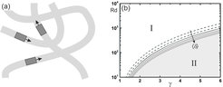
In this diagram, we find two qualitatively different regions, labeled I and II. These are separated by a boundary which depends on the average detours we impose on the customers. The solid curve corresponds to a detour of 1.5 (i.e., rides are on average 1.5 times as long as the direct route). In region I, the market competition leads to two stable fixed points. One corresponds to the ride sharing system serving only a niche market at high price and low demand. On the other, the ride sharing system out-competes all others. In region II, there is only one stable fixed point, corresponding to the niche market scenario. It is important to note that while Rd is usual on the order of a few thousand in big cities, it reaches only a few hundred in rural areas. For a mini-bus with driver, γ is about 4 or 5, such that ride sharing is not easily deployed there at break-even conditions. However, for autonomous vehicles, where no driver’s salary is required, γ lies between 1 and 2, close to the left boundary of the figure. Hence ride sharing may win the competition against the private car even in rural areas if autonomous driving is implemented.
References
[1] M. Ballerini, N. Cabibbo, R. Candelier, A. Cavagna, E. Cisbani, I. Giardina, V. Lecomte, A. Orlandi, G. Parisi, A. Procaccini, M. Viale and V. Zdravkovic, P.N.A.S. 105 (2008) 1232.
[2] A. Attanasi, A. Cavagna, L. Del Castello, I. Giardina, T.S. Grigera, A. Jelić, S. Melillo, L. Parisi, O. Pohl, E. Shen and M. Viale, Nat. Phys. 10 (2014) 691.
[3] E. Ben-Jacob, I. Cohen and H. Levine, Adv. Phys. 49 (2000) 395.
[4] T. Vissers, A. Wysocki, M. Rex, H. Löwen, C.P. Royall, A. Imhofa and A. van Blaaderena, Soft Matter 7 (2011) 2352.
[5] C.W. Meyer, G. Ahlers and D.S. Cannell, Phys. Rev. Lett. 59 (1987) 1577.
[6] M.C. Cross and P.C. Hohenberg, Rev. Mod. Phys. 65 (1993) 851.
[7] D. Helbing, Rev. Mod. Phys.73 (2001) 1067.
[8] A. Sokolov, I.S. Aranson, J.O. Kessler and R.E. Goldstein, Phys. Rev. Lett. 98 (2007) 158102.
[9] H.H. Wensink, J. Dunkel, S. Heidenreich, K. Drescher, R.E. Goldstein, H. Löwen and J.M. Yeomans, P.N.A.S. 109 (2012) 14308.
[10] A. Kolmogoroff, Math. Annalen 112 (1936) 155.
[11] R.K.P. Zia and B. Schmittmann, J. Stat. Mech.: TheoryExp. (2007) P07012.
[12] G. Kirchhoff, Ann. Phys. 151 (1848) 189.
[13] E. T. Jaynes, Annu. Rev. Phys. Chem. 31 (1980) 579.
[14] C. Maes and K. Netocny, J. Math. Phys. 48 (2007) 053306.
[15] P. Glansdorff and I. Prigogine, Thermodynamic theory of structure, stability, and fluctuations (Wiley, London 1971).
[16] L.M. Martyushev and V.D. Seleznev, Phys. Rep. 426 (2006) 1.
[17] J. Keizer and R.F. Fox, P.N.A.S. 71 (1974) 192.
[18] R. Landauer, Phys. Rev. A 12 (1975) 636.
[19] G. Nicolis, Rep. Prog. Phys. 42 (1979) 225.
[20] S. Kalpazidou, Ann. Prob.23 (1995) 966.
[21] B. Altaner, S. Grosskinsky, S. Herminghaus, L. Katthän, M. Timme and J. Vollmer, Phys. Rev. E 85 (2012) 041133.
[22] K. Roeller, J. Vollmer and S. Herminghaus, Chaos 19 (2009) 041106.
[23] S. Ulrich, T. Aspelmeier, K. Roeller, A. Fingerle, S. Herminghaus and A. Zippelius, Phys. Rev. Lett. 102 (2009) 148002.
[24] J.P.D. Clewett, K. Roeller, R.M. Bowley, S. Herminghaus, and M.R. Swift, Phys. Rev. Lett. 109 (2012) 228002.
[25] S. Herminghaus and M.G. Mazza, Soft Matter 13 (2017) 898.
[26] C. Krüger, C. Bahr, S. Herminghaus and C.C. Maass, Eur. Phys. J. E 39 (2016) 64.
[27] A. D. Wiesner-Gross and C. E. Freer, Phys. Rev. Lett. 110 (2013) 168702.